Data Augmentation: Case Study in Deep Learning with TensorFlow

Introduction : What is data augmentation
Data augmentation is a technique used in machine learning to automatically generate additional training data through transformations that produce data similar to real data.
This technique is useful for scenarios where it is technically complex or even expensive to collect real data, such as in the fields of health, security or space research.
Also, in cases where training data is limited or of poor quality, such an implementation allows the creation of new data that can improve the performance of the machine learning model.
The objective of data augmentation is to introduce other aspects of the data to the model to allow for better generalisation.
Case study
Let’s look at an example where the rate of correct answers stagnates too quickly:
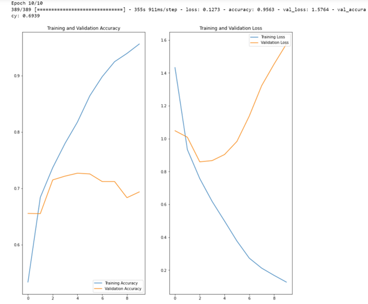
NB : x=number of epochs, y=percentage of accuracy
The graph above shows that the training accuracy of our model, in blue, increases linearly over the learning cycles (epochs), while the validation accuracy, in orange, stagnates.
Moreover, the accuracy gap between training and validation accuracy only increases from the second cycle onwards: we are confronted here with the problem of overlearning.
Note that the less training data we have, the faster this overlearning phenomenon occurs.
We are therefore going to try to solve this problem of overlearning by increasing the amount of data, by using the keras pre-processing layers:
tf.keras.layers.RandomFlip ,
tf.keras.layers.RandomRotation
tf.keras.layers.RandomZoom
from tensorflow import keras
data_augmentation = keras.Sequential(
  [
    layers.RandomFlip("horizontal",
                      input_shape=(img_height,
                                  img_width,
                                  3)),
    layers.RandomZoom(0.1),
  ]
)
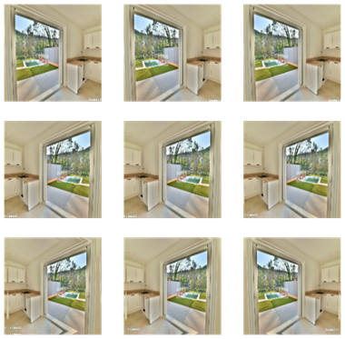
Here we have created a small sequence of two simple image treatments:
• A horizontal “flip” (inversion) ;
• A random zoom up to 10%.
The script below shows us 9 versions of the first image in our training set:
plt.figure(figsize=(10, 10))
for images, _ in train_ds.take(1):
  for i in range(9):
    augmented_images = data_augmentation(images)
    ax = plt.subplot(3, 3, i + 1)
    plt.imshow(augmented_images[0].numpy().astype("uint8"))
    plt.axis("off")
We restart the learning of our neural network:
model = tf.keras.Sequential([
    data_augmentation,
    layers.experimental.preprocessing.Rescaling(1. / 255),
    layers.Conv2D(64, (3, 3), padding='same', activation='relu'),
    layers.MaxPooling2D((2, 2)),
    layers.Conv2D(64, (3, 3), padding='same', activation='relu'),
    layers.MaxPooling2D((2, 2)),
    layers.Conv2D(128, (3, 3), padding='same', activation='relu'),
    layers.MaxPooling2D((2, 2)),
    layers.Conv2D(128, (3, 3), padding='same', activation='relu'),
    layers.MaxPooling2D((2, 2)),
    layers.Dropout(0.5),
    layers.Flatten(),
    layers.Dense(128, activation='relu'),
    layers.Dense(num_classes)
    ])
Note in passing that we abandon learning as soon as there is a 50% difference between learning and validation rates, in order to shorten learning:
• this is sufficient to check that the number of “useful” learning cycles has increased ;
• this abandonment avoids, whatever the correct answer rates, the phenomenon of overlearning.
Let us compile the model:
model.compile(optimizer='adam',
              loss=tf.keras.losses.SparseCategoricalCrossentropy(from_logits=True),
              metrics=['accuracy'])
model.summary()
Model: "sequential_2"
_________________________________________________________________
 Layer (type)                Output Shape              Param #
=================================================================
 sequential_1 (Sequential)   (None, 180, 180, 3)       0

 rescaling_2 (Rescaling)     (None, 180, 180, 3)       0

 conv2d_4 (Conv2D)           (None, 180, 180, 64)      1792

 max_pooling2d_4 (MaxPooling  (None, 90, 90, 64)       0
 2D)

 conv2d_5 (Conv2D)           (None, 90, 90, 64)        36928

 max_pooling2d_5 (MaxPooling  (None, 45, 45, 64)       0
 2D)

 conv2d_6 (Conv2D)           (None, 45, 45, 128)       73856

 max_pooling2d_6 (MaxPooling  (None, 22, 22, 128)      0
 2D)

 conv2d_7 (Conv2D)           (None, 22, 22, 128)       147584

 max_pooling2d_7 (MaxPooling  (None, 11, 11, 128)      0
 2D)

 dropout_1 (Dropout)         (None, 11, 11, 128)       0

 flatten_1 (Flatten)         (None, 15488)             0

 dense_2 (Dense)             (None, 128)               1982592

 dense_3 (Dense)             (None, 13)                1677

=================================================================
Total params: 2,244,429
Trainable params: 2,244,429
Non-trainable params: 0
_________________________________________________________________
Let’s train the model, with a maximum of 15 training cycles:
epochs =15
history = model.fit(
  train_ds,
  validation_data=val_ds,
  epochs=epochs
)
The script below allows us to display the learning and validation curves:
acc = history.history['accuracy']
val_acc = history.history['val_accuracy']
loss = history.history['loss']
val_loss = history.history['val_loss']
epochs_range = range(epochs)
plt.figure(figsize=(8, 8))
plt.subplot(1, 2, 1)
plt.plot(epochs_range, acc, label='Training Accuracy')
plt.plot(epochs_range, val_acc, label='Validation Accuracy')
plt.legend(loc='lower right')
plt.title('Training and Validation Accuracy')
plt.subplot(1, 2, 2)
plt.plot(epochs_range, loss, label='Training Loss')
plt.plot(epochs_range, val_loss, label='Validation Loss')
plt.legend(loc='upper right')
plt.title('Training and Validation Loss')
plt.show()
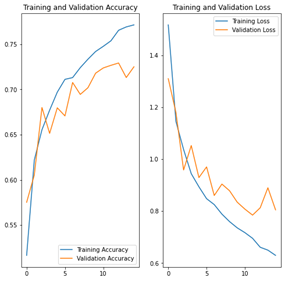
NB : x=number of epochs, y=percentage accuracy
We notice less overfitting than before, and the accuracy rates in training and validation remain very close until about 10 training cycles. Moreover, the difference does not visibly reach 50% after the 15th and last cycle.
Finally, let us compare the results of the models without and with augmentation by categorising an image not included in the training or validation set:
from pathlib import Path
imag_path="C:/Users/DataMindset/Downloads/deep_learning_images_2022_10_04/deep_learning_images/TEST image 2 novembre/fenetre/8.jpg
img = tf.keras.utils.load_img(
    imag_path, target_size=(img_height, img_width)
)
img_array = tf.keras.utils.img_to_array(img)
img_array = tf.expand_dims(img_array, 0) # Create a batch
predictions = model.predict(img_array)
score = tf.nn.softmax(predictions[0])
print(
    "This image looks more like the {} category at {:.2f} per cent."
    .format(class_names[np.argmax(score)], 100 * np.max(score))
)
With the “initial without increase” model, we get:
Sortie : 1/1 [=============================] – 0s 44ms/pas
This image is more like the window category at 64.96 per cent.
With the “augmented” model, we get :
Sortie : 1/1 [=============================] – 0s 44ms/pas
This image looks more like the window category at 94.69 per cent.
Conclusion
In conclusion, data augmentation gives us better results for two reasons:
• We can increase the number of learning cycles without overlearning.
• This results in a better categorisation of the test data.


